
Documents Live, a web authoring and publishing system
Documents Live, a web authoring and publishing system
If you see this, something is wrong
First published on Saturday, Jul 6, 2024 and last modified on Thursday, Apr 10, 2025
Mathedu SAS
The usual manner to reference vectors is their cartesian coordinates in the canonical base.
But in the euclidean plane \( \mathbb{P}\) , the canonical base is orthonormal and we can define angles between vectors.
Because of that, we may define another powerful mean to reference non-zero vectors, the polar coordinates, made of its norm \( R\) and its angle with the \( x\) axis \( \theta\) .
And the polar coordinates are very useful to manipulate angles between non-zero vectors, as well as to define and manipulate rotations in the euclidean plane \( \mathbb{P}\) .
The present note let you discover all these topics.
The non-zero vectors don’t only have cartasion coordinates, they may also be defined by a length and an angle, their polar coordinates.
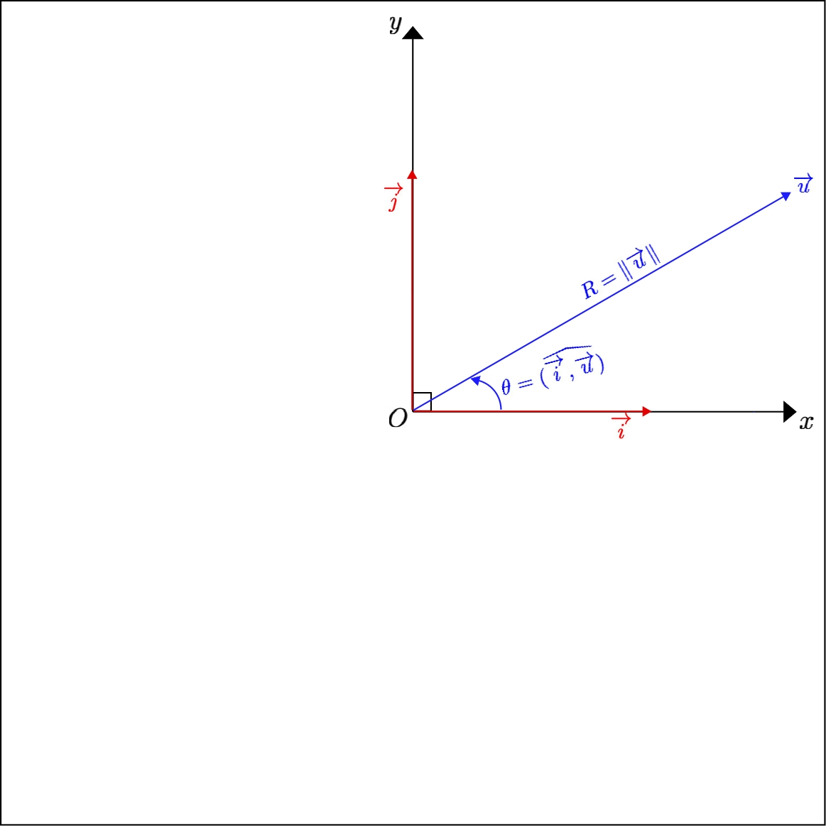
Definition 1
Assume \( \overrightarrow{u}\in\mathbb{P}^*\) is a non zero vector.
Then its polar coordinates in the canonical orthonormal base \( (\overrightarrow{i},\overrightarrow{j})\) are defined as:
Theorem 1
Assume \( \overrightarrow{u}\in\mathbb{P}^*\) is a non zero vector.
Assume its polar coordinates in the canonical orthonormal base \( (\overrightarrow{i},\overrightarrow{j})\) are \( R\) and \( \theta\) .
Then its cartesian coordinates in the base \( (\overrightarrow{i},\overrightarrow{j})\) are:
Proof
Assume \( \overrightarrow{u}\in\mathbb{P}^*\) is a non zero vector.
Assume its polar coordinates in the canonical orthonormal base \( (\overrightarrow{i},\overrightarrow{j})\) are \( R\) and \( \theta\) .
Consider the unit vector \( \overrightarrow{u}_0=\frac{\overrightarrow{u}}{R}\) .
Then, as \( \theta=(\widehat{\overrightarrow{i},\overrightarrow{u}})=(\widehat{\overrightarrow{i},\overrightarrow{u}_{0}})\) , \( \overrightarrow{u}_{0}\) is equal to the column vector \( \overrightarrow{u}_0=\begin{bmatrix} \cos(\theta)\\\sin(\theta)\end{bmatrix}\) .
Consequently, as \( \overrightarrow{u}=R\overrightarrow{u}_{0}\) , \( \overrightarrow{u}\) is equal to the column vector \( \overrightarrow{u}=\begin{bmatrix} R\cos(\theta)\\R\sin(\theta)\end{bmatrix}\) , and cartesian its coordinates are:
As a consequence of the theorem 1, if the cartesian coordinates of the non zero vector \( \overrightarrow{u}\in\mathbb{P}^*\) are \( x\) and \( y\) , then the following formulae apply for its polar coordinates \( R\) and \( \theta\) :
\( R=\sqrt{x^{2}+y^{2}}\) ,
\( \cos(\theta)=\frac{x}{R}\) ,
and \( \sin(\theta)=\frac{y}{R}\) .
The following examples deduce the polar angles of the vectors from their cosine and sine, as they were part of the examples given in the lecture 24 about the trigonometry in the unit circle.
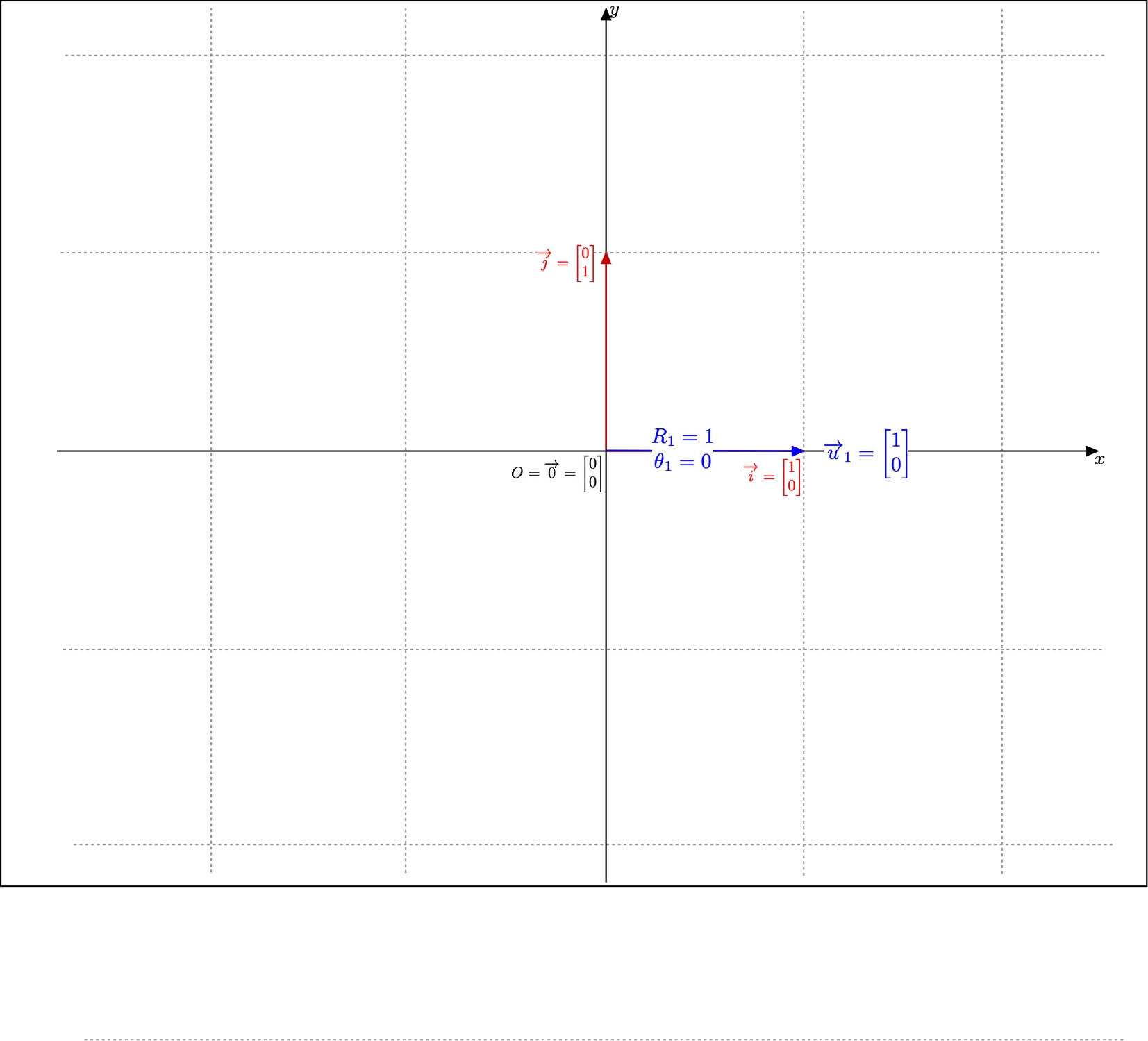
The first example is \( \overrightarrow{u}_{1}=\begin{bmatrix}1\\0\end{bmatrix}\) .
The cartesian coordinates of \( \overrightarrow{u}_{1}\) are:
its abscissa \( x_{1}=1\) ,
and its ordinate \( y_{1}=0\)
Its norm is \( R_{1}=\sqrt{1^{2}+0^{2}}=1\) .
So that the cosine and sine of its polar angle are:
\( \cos(\theta_{1})=\frac{1}{1}=1\) ,
and \( \sin(\theta_{1})=\frac{0}{1}=0\) .
Consequently, its polar angle is \( \theta_{1}=0\) modulo \( 2\pi\) .
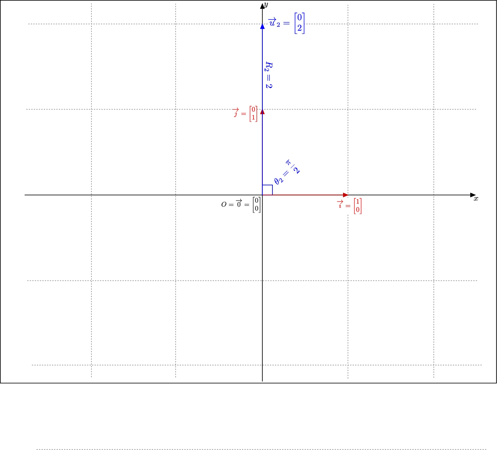
The second example is \( \overrightarrow{u}_{2}=\begin{bmatrix}0\\2\end{bmatrix}\) .
The cartesian coordinates of \( \overrightarrow{u}_{2}\) are:
its abscissa \( x_{2}=0\) ,
and its ordinate \( y_{2}=2\)
Its norm is \( R_{2}=\sqrt{0^{2}+2^{2}}=\sqrt{4}=2\) .
So that the cosine and sine of its polar angle are:
\( \cos(\theta_{2})=\frac{0}{2}=0\) ,
and \( \sin(\theta_{2})=\frac{2}{2}=1\) .
Consequently, its polar angle is \( \theta_{2}=\frac{\pi}{2}\) modulo \( 2\pi\) .
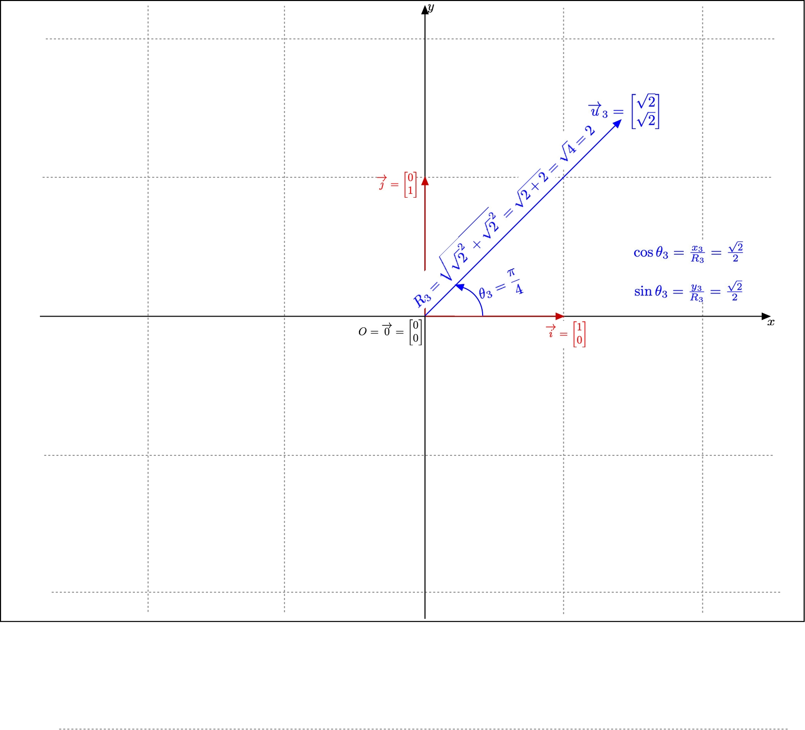
The third example is \( \overrightarrow{u}_{3}=\begin{bmatrix}\sqrt{2}\\\sqrt{2}\end{bmatrix}\) .
The cartesian coordinates of \( \overrightarrow{u}_{3}\) are:
its abscissa \( x_{3}=\sqrt{2}\) ,
and its ordinate \( y_{3}=\sqrt{2}\)
Its norm is \( R_3=\sqrt{\sqrt{2}^2+\sqrt{2}^2}=\sqrt{2+2}=\sqrt{4}=2\) .
So that the cosine and sine of its polar angle are:
\( \cos(\theta_{2})=\frac{\sqrt{2}}{2}\) ,
and \( \sin(\theta_{2})=\frac{\sqrt{2}}{2}\) .
Consequently, its polar angle is \( \theta_{3}=\frac{\pi}{4}\) modulo \( 2\pi\) .
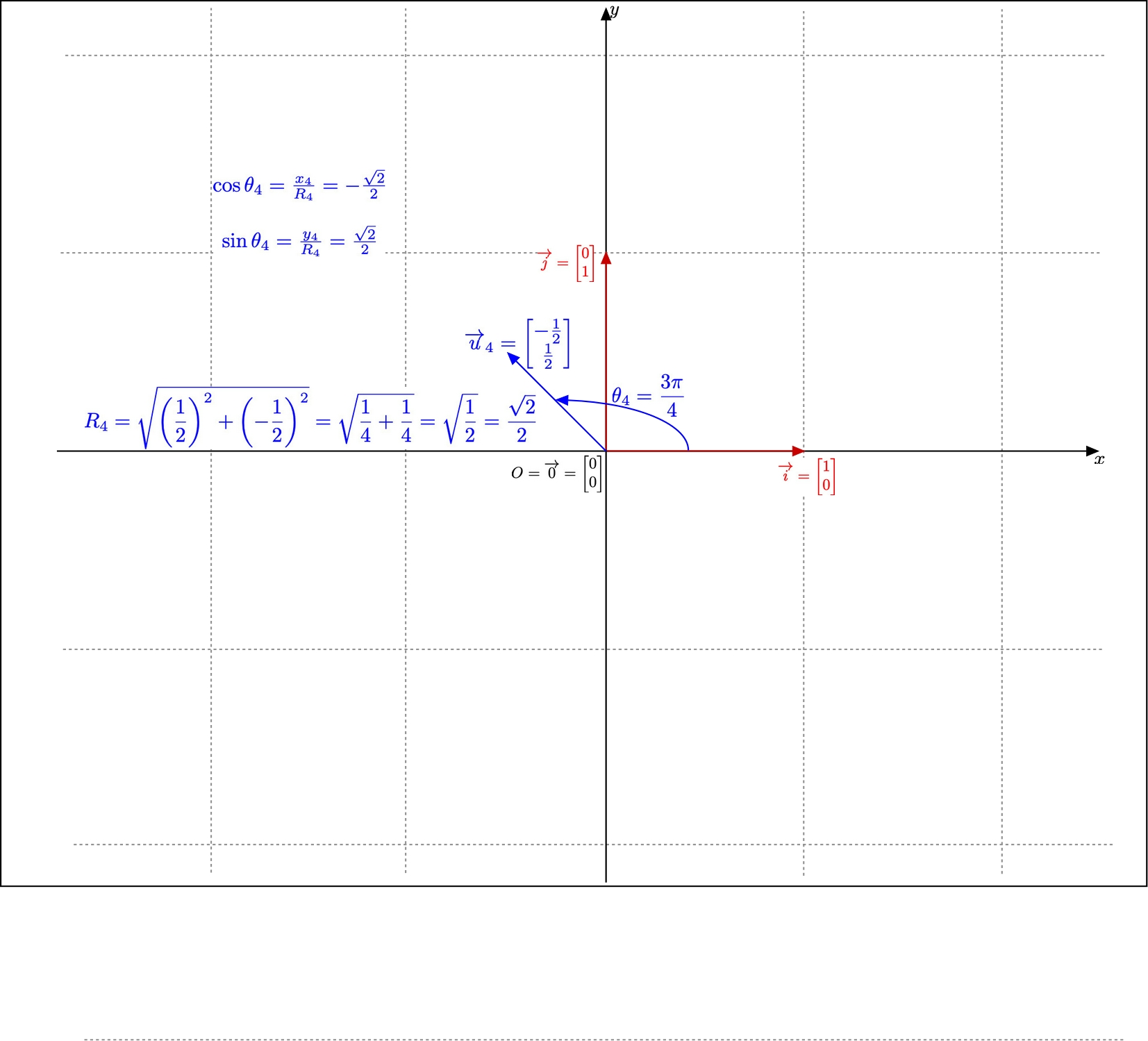
The fourth example is \( \overrightarrow{u}_4=\begin{bmatrix}\frac{1}{2}\\{-\frac{1}{2}}\end{bmatrix}\) .
The cartesian coordinates of \( \overrightarrow{u}_{4}\) are:
its abscissa \( x_{4}=-\frac{1}{2}\) ,
and its ordinate \( y_{4}=\frac{1}{2}\)
Its norm is \( R_4=\sqrt{\frac{1}{2}^2+\left(-\frac{1}{2}\right)^2} =\sqrt{\frac{1}{4}+\frac{1}{4}}=\sqrt{\frac{1}{2}}=\frac{\sqrt{2}}{2}\) .
So that the cosine and sine of its polar angle are:
\( \cos(\theta_{4})=\frac{-\frac{1}{2}}{\frac{\sqrt{2}}{2}}=-\frac{1}{\sqrt{2}}=-\frac{\sqrt{2}}{2}\) ,
and \( \sin(\theta_{4})=\frac{\frac{1}{2}}{\frac{\sqrt{2}}{2}}=\frac{1}{\sqrt{2}}=\frac{\sqrt{2}}{2}\) .
Consequently, its polar angle is \( \theta_{4}=\frac{3\pi}{4}\) modulo \( 2\pi\) .
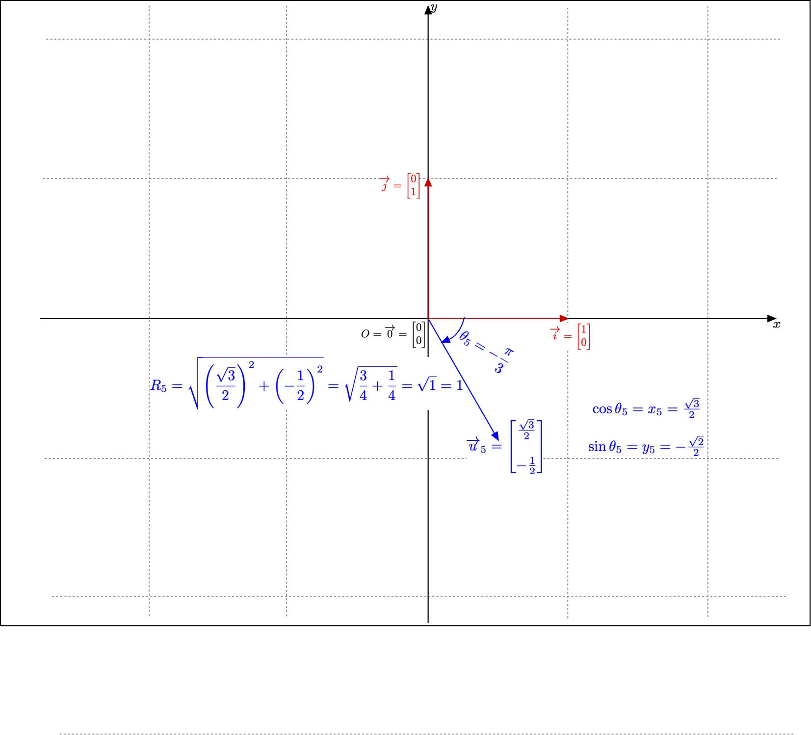
The fifth example is \( \overrightarrow{u}_5=\begin{bmatrix}\frac{\sqrt{3}}{2}\\{-\frac{1}{2}}\end{bmatrix}\) .
The cartesian coordinates of \( \overrightarrow{u}_{5}\) are:
its abscissa \( x_{5}=\frac{\sqrt{3}}{2}\) ,
and its ordinate \( y_{5}=-\frac{1}{2}\)
Its norm is \( R_5=\sqrt{\left(\frac{\sqrt{3}}{2}\right)^2+\left(-\frac{1}{2}\right)^2} =\sqrt{\frac{3}{4}+\frac{1}{4}}=\sqrt{1}=1\) .
So that the cosine and sine of its polar angle are:
\( \cos(\theta_{5})=\frac{\frac{\sqrt{3}}{2}}{1}=\frac{\sqrt{3}}{2}\) ,
and \( \sin(\theta_{4})=\frac{-\frac{1}{2}}{1}=-\frac{1}{2}\) .
Consequently, its polar angle is \( \theta_{5}=-\frac{\pi}{3}\) modulo \( 2\pi\) .
Particular configurations of the polar angles of two vectors correspond to particular, aligned or orthogonal, configurations of these vectors.
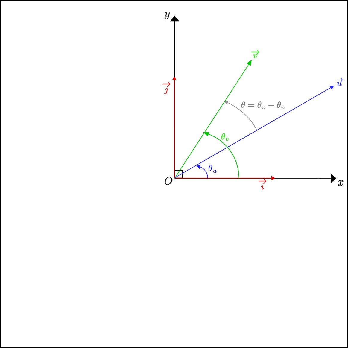
Theorem 2
Assume \( (\overrightarrow{u},\overrightarrow{v})\in(\mathbb{P}^*)^2\) are non zero vectors with polar angles \( \theta_{u}\) and \( \theta_{v}\) .
Then the angle \( (\widehat{\overrightarrow{u},\overrightarrow{v}})\) is equal to \( \theta=\theta_v-\theta_u\) modulo \( 2\pi\) .
Proof
Assume \( (\overrightarrow{u},\overrightarrow{v})\in(\mathbb{P}^*)^2\) are non zero vectors with polar angles \( \theta_{u}\) and \( \theta_{v}\) .
Let’s denote \( \theta=(\widehat{\overrightarrow{u},\overrightarrow{v}})\) .
Then \( \theta_{u}=(\widehat{\overrightarrow{i},\overrightarrow{u}})\) and \( \theta_{v}=(\widehat{\overrightarrow{i},\overrightarrow{v}})\) .
Consequently, by definition of \( (\widehat{\overrightarrow{u},\overrightarrow{v}})\) , \( \theta=\theta_v-\theta_u\) modulo \( 2\pi\) .

Assume \( (\overrightarrow{u},\overrightarrow{v})\in(\mathbb{P}^*)^2\) are non zero vectors with polar angles \( \theta_{u}\) and \( \theta_{v}\) .
Assume \( \theta_v=\theta_u\) or, more precisely, \( \theta_v\equiv\theta_u\mod 2\pi\) .
Then the angle \( (\widehat{\overrightarrow{u},\overrightarrow{v}})\) is equal to \( \theta=\theta_v-\theta_u=0\) modulo \( 2\pi\) .
Consequently, \( \overrightarrow{u}\) and \( \overrightarrow{v}\) are positively aligned.
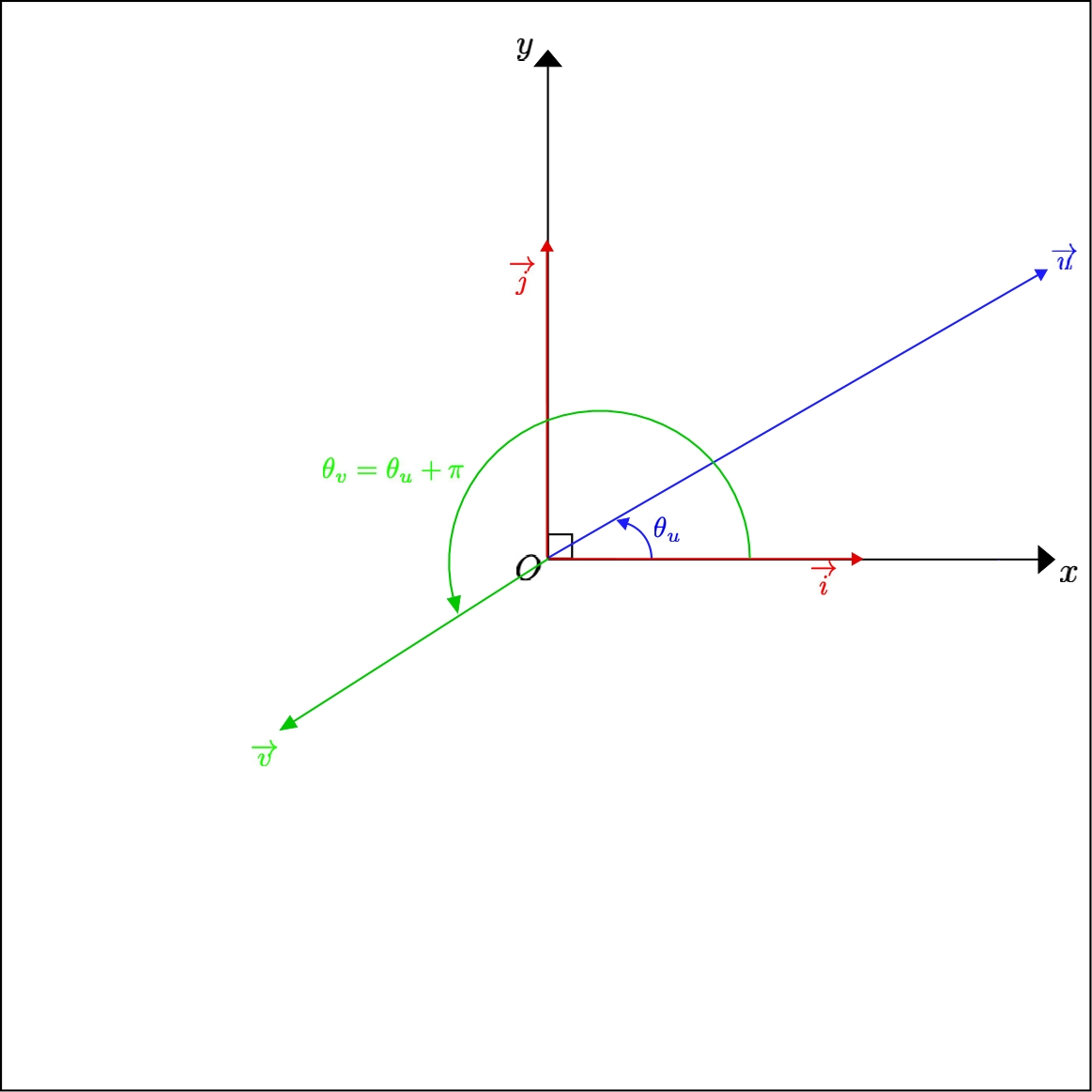
Assume \( (\overrightarrow{u},\overrightarrow{v})\in(\mathbb{P}^*)^2\) are non zero vectors with polar angles \( \theta_{u}\) and \( \theta_{v}\) .
Assume \( \theta_v=\theta_u+\pi\) or, more precisely, \( \theta_v\equiv\theta_u+\pi\mod 2\pi\) .
Then the angle \( (\widehat{\overrightarrow{u},\overrightarrow{v}})\) is equal to \( \theta=\theta_v-\theta_u=\pi\) modulo \( 2\pi\) .
Consequently, \( \overrightarrow{u}\) and \( \overrightarrow{v}\) are negatively aligned.

Assume \( (\overrightarrow{u},\overrightarrow{v})\in(\mathbb{P}^*)^2\) are non zero vectors with polar angles \( \theta_{u}\) and \( \theta_{v}\) .
Assume \( \theta_v=\theta_u+\frac{\pi}{2}\) or, more precisely, \( \theta_v\equiv\theta_u+\frac{\pi}{2}\mod 2\pi\) .
Then the angle \( (\widehat{\overrightarrow{u},\overrightarrow{v}})\) is equal to \( \theta=\theta_v-\theta_u=\frac{\pi}{2}\) modulo \( 2\pi\) .
Consequently and by definition, \( \overrightarrow{u}\) and \( \overrightarrow{v}\) are orthogonal in the direct direction.
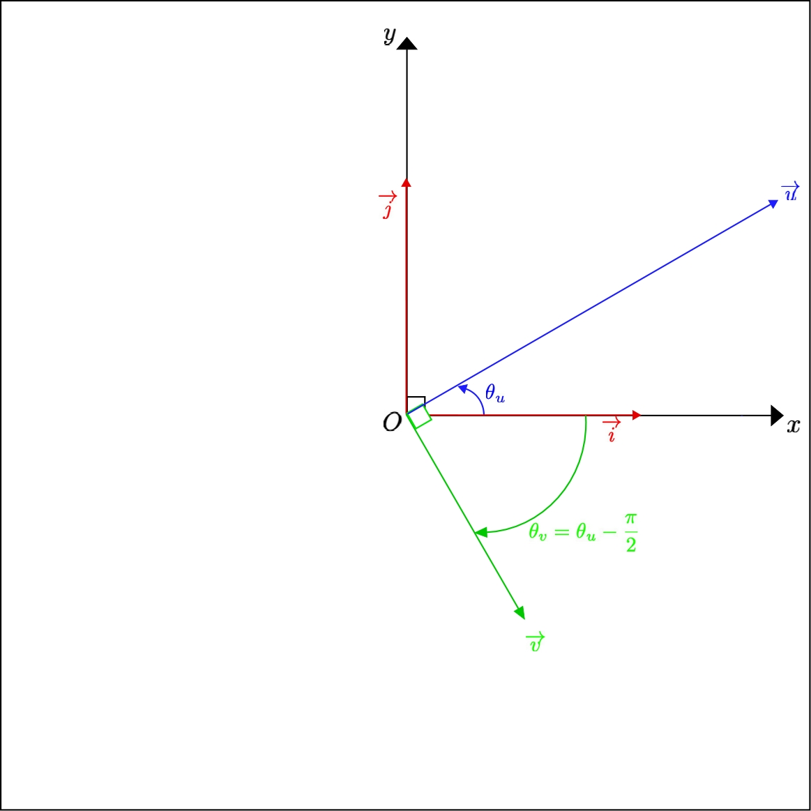
Assume \( (\overrightarrow{u},\overrightarrow{v})\in(\mathbb{P}^*)^2\) are non zero vectors with polar angles \( \theta_{u}\) and \( \theta_{v}\) .
Assume \( \theta_v=\theta_u-\frac{\pi}{2}\) or, more precisely, \( \theta_v\equiv\theta_u-\frac{\pi}{2}\mod 2\pi\) .
Then the angle \( (\widehat{\overrightarrow{u},\overrightarrow{v}})\) is equal to \( \theta=\theta_v-\theta_u=-\frac{\pi}{2}\) modulo \( 2\pi\) .
Consequently and by definition, \( \overrightarrow{u}\) and \( \overrightarrow{v}\) are orthogonal in the reverse direction.
Now we shall use the ‘arccosine’ and ‘arcsine’ inverse trigonometric functions to convert cartesian coordinates of a non-zero vector into its polar coordinates.
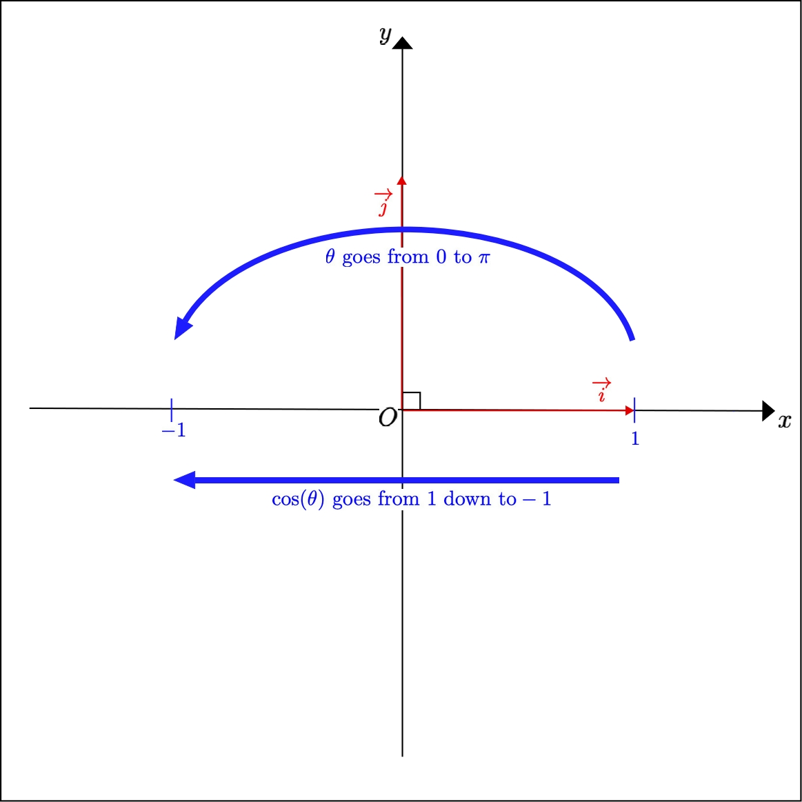
When \( \theta\) goes from \( 0\) to \( \pi\) , \( \cos(\theta)\) goes from \( 1\) down to \( -1\) .
Consequently, the cosine function is one to one from \( [0,\pi]\) onto \( [-1,1]\) .
We define the function ‘arccosine’ as the inverse of the cosine function restricted to \( [0,\pi]\) .
That is that, for any \( x\in[-1,1]\) , \( \arccos(x)\) is the angle \( \theta\in[0,\pi]\) so that \( \cos(\theta)=x\) .

When \( \theta\) goes from \( -\frac{\pi}{2}\) to \( \frac{\pi}{2}\) , \( \sin(\theta)\) goes from \( -1\) to \( 1\) .
Consequently, the sine function is one to one from \( \left[-\frac{\pi}{2},\frac{\pi}{2}\right]\) onto \( [-1,1]\) .
We define the function ‘arcsine’ as the inverse of the sine function restricted to \( \left[-\frac{\pi}{2},\frac{\pi}{2}\right]\) .
That is that, for any \( x\in[-1,1]\) , \( \arcsin(x)\) is the angle \( \theta\in\left[-\frac{\pi}{2},\frac{\pi}{2}\right]\) so that \( \sin(\theta)=x\) .
Assume \( (x,y)\in\mathbb{R}^2\) are the cartesian coordinates of a unit vector \( \overrightarrow{u}\) , that are so that \( x^2+y^2=1\) , \( -1\le x\le 1\) and \( -1\le y\le 1\) .

If the unit vector \( \overrightarrow{u}\) is on the \( x^{+}\) semi-axis, then its abscissa is equal to \( 1\) and its ordinate is equal to \( 0\) .
Consequently, \( \overrightarrow{u}=\overrightarrow{i}\) , and its polar angle is \( \theta=\widehat{(\overrightarrow{i},\overrightarrow{i})}=0\) modulo \( 2\pi\) .
As that angle is between \( 0\) and \( \pi\) , and as \( \cos(\theta)=x\) , we have \( \theta=\arccos(x)\) .
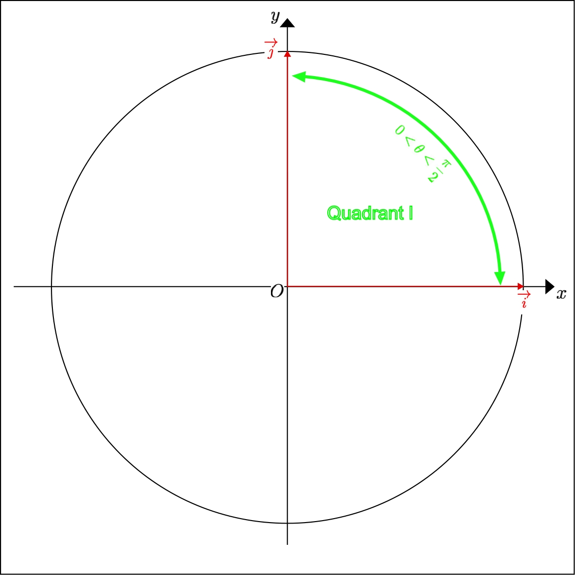
If the unit vector \( \overrightarrow{u}\) is in the first quadrant of the unit circle, then its abscissa and ordinate are strictly comprised between \( 0\) and \( 1\) and its polar angle is strictly comprised between \( 0\) and \( \frac{\pi}{2}\) .
The polar angle is thus between \( 0\) and \( \pi\) , and \( \cos(\theta)=x\) , so that \( \theta=\arccos(x)\) .

If the unit vector \( \overrightarrow{u}\) is on the \( y^{+}\) semi-axis, then its abscissa is equal to \( 0\) and its ordinate is equal to \( 1\) .
Consequently, \( \overrightarrow{u}=\overrightarrow{j}\) , and its polar angle is \( \theta=\widehat{(\overrightarrow{i},\overrightarrow{j})}=\frac{\pi}{2}\) modulo \( 2\pi\) .
As that angle is between \( 0\) and \( \pi\) , and as \( \cos(\theta)=x\) , we have \( \theta=\arccos(x)\) .
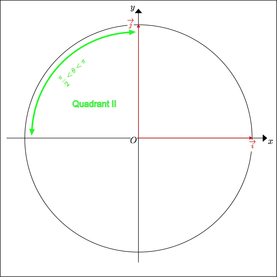
If the unit vector \( \overrightarrow{u}\) is in the second quadrant of the unit circle, then its abscissa strictly comprised between \( -1\) and \( 0\) , its ordinate is strictly comprised between \( 0\) and \( 1\) , and its polar angle is strictly comprised between \( \frac{\pi}{2}\) and \( \pi\) .
The polar angle is thus between \( 0\) and \( \pi\) , and \( \cos(\theta)=x\) , so that \( \theta=\arccos(x)\) .
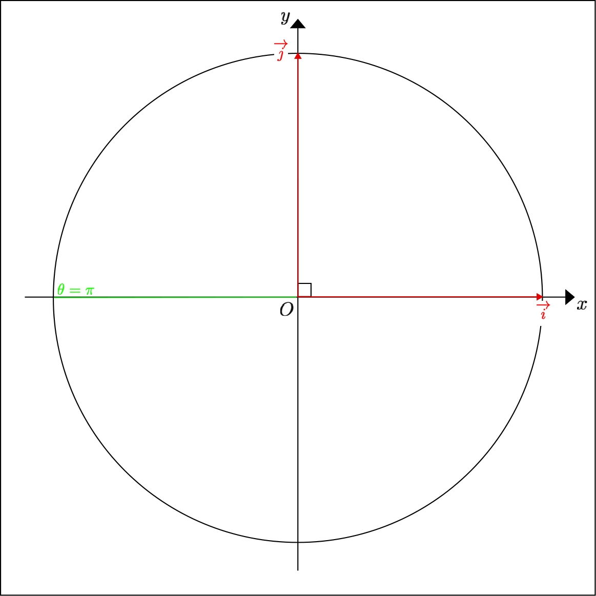
If the unit vector \( \overrightarrow{u}\) is on the \( x^{-}\) semi-axis, then its abscissa is equal to \( -1\) and its ordinate is equal to \( 0\) .
Consequently, \( \overrightarrow{u}=-\overrightarrow{i}\) , and its polar angle is \( \theta=\widehat{(\overrightarrow{i},-\overrightarrow{i})}=\pi\) modulo \( 2\pi\) .
As that angle is between \( 0\) and \( \pi\) , and as \( \cos(\theta)=x\) , we have \( \theta=\arccos(x)\) .
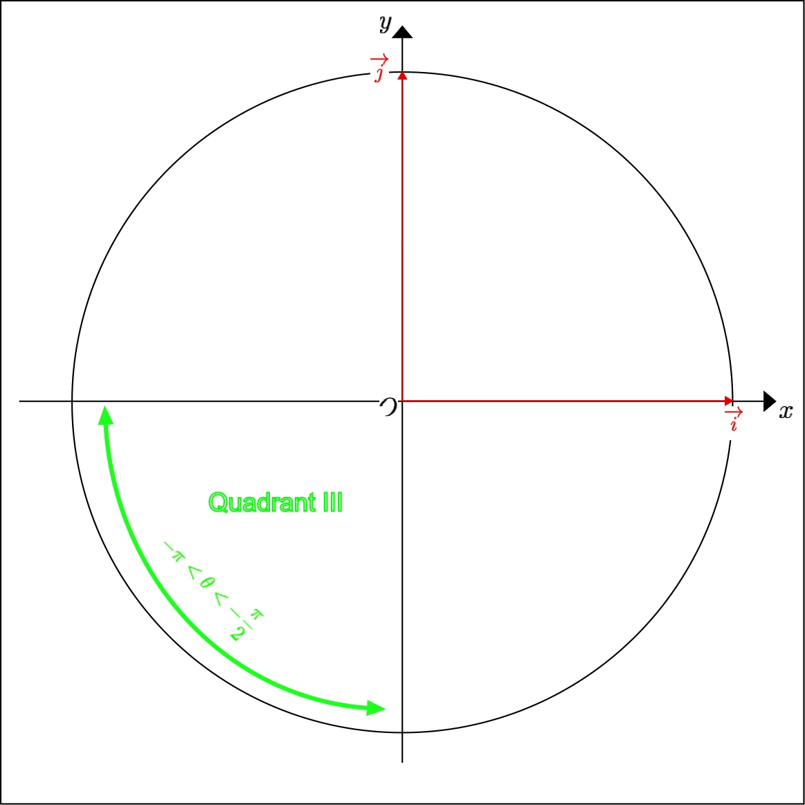
If the unit vector \( \overrightarrow{u}\) is in the third quadrant of the unit circle, then its abscissa and ordinate are strictly comprised between \( -1\) and \( 0\) and its polar angle \( \theta\) is strictly comprised between \( -\pi\) and \( -\frac{\pi}{2}\) .
The angle \( \theta+\pi\) is thus between \( 0\) and \( \pi\) and is so that
\( \cos(\theta+\pi)=-\cos(\theta)=-x\) .
Consequently, \( \theta=\arccos(-x)-\pi\) .

If the unit vector \( \overrightarrow{u}\) is on the \( y^{-}\) semi-axis, then its abscissa is equal to \( 0\) and its ordinate is equal to \( -1\) .
Consequently, \( \overrightarrow{u}=-\overrightarrow{j}\) , and its polar angle is \( \theta=\widehat{(\overrightarrow{i},-\overrightarrow{j})}=-\frac{\pi}{2}\) modulo \( 2\pi\) .
As that angle is between \( -\frac{\pi}{2}\) and \( \frac{\pi}{2}\) , and as \( \sin(\theta)=y\) , we have \( \theta=\arcsin(y)\) .
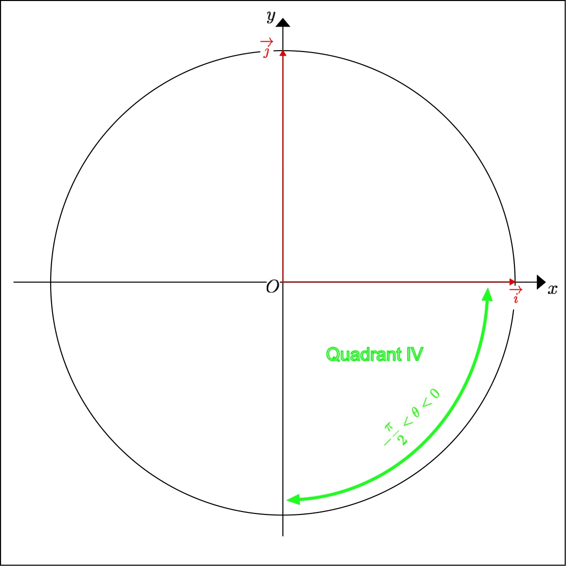
If the unit vector \( \overrightarrow{u}\) is in the fourth quadrant of the unit circle, then its abscissa strictly comprised between \( 0\) and \( 1\) , its ordinate is strictly comprised between \( -1\) and \( 10\) , and its polar angle is strictly comprised between \( -\frac{\pi}{2}\) and \( 0\) .
The polar angle is thus between \( -\frac{\pi}{2}\) and \( \frac{\pi}{2}\) , and \( \sin(\theta)=y\) , so that \( \theta=\arcsin(y)\) .
The table 1 recapitulates the calculation of the polar angles of unit vectors, depending on their geometrical configurations.
| Abscissa Range | Ordinate Range | Polar Angle | Polar Angle Range | |
| \( x^{+}\) semi-axis | \( x=1\) | \( y=0\) | \( \theta=\arccos(x)\) | \( \theta=0\) |
| Quadrant I | \( 0<x<1\) | \( 0<y<1\) | \( \theta=\arccos(x)\) | \( 0<\theta<\frac{\pi}{2}\) |
| \( y^{+}\) semi-axis | \( x=0\) | \( y=1\) | \( \theta=\arccos(x)\) | \( \theta=\frac{\pi}{2}\) |
| Quadrant II | \( -1<x<0\) | \( 0<y<1\) | \( \theta=\arccos(x)\) | \( \frac{\pi}{2}<\theta<\pi\) |
| \( x^{-}\) semi-axis | \( x=-1\) | \( y=0\) | \( \theta=\arccos(x)\) | \( \theta=\pi\) |
| Quadrant III | \( -1<x<0\) | \( -1<y<0\) | \( \theta=\arccos(-x)-\pi\) | \( -\pi<\theta<-\frac{\pi}{2}\) |
| \( y^{-}\) semi-axis | \( x=0\) | \( y=-1\) | \( \theta=\arcsin(y)\) | \( \theta=-\frac{\pi}{2}\) |
| Quadrant IV | \( 0<x<1\) | \( -1<y<0\) | \( \theta=\arcsin(y)\) | \( -\frac{\pi}{2}<\theta<0\) |
Assume \( (x,y)\in\mathbb{R}^2\) are the cartesian coordinates of a non zero vector \( \overrightarrow{u}\in\mathbb{P}^*\) .
Then the norm of \( \overrightarrow{u}\) is equal to \( R=\sqrt{x^2+y^2}\) and its polar angle is equal to the polar angle of the unit vector \( \overrightarrow{u}_{0}=\frac{\overrightarrow{u}}{R}=\frac{\overrightarrow{u}}{\sqrt{x^2+y^2}}\) , which abscissa is \( x_{0}=\frac{x}{\sqrt{x^2+y^2}}\) and ordinate is \( y_{0}=\frac{y}{\sqrt{x^2+y^2}}\) .
Consequently, the table of conversion of cartesian coordinates to polar coordiantes of a non zero vector may be deduced from table 1.
| Abscissa Range | Ordinate Range | Norm | Polar Angle | Polar Angle Range | |
| \( x^{+}\) semi-axis | \( x>0\) | \( y=0\) | \( R=x\) | \( \theta=\arccos\left(\frac{x}{\sqrt{x^2+y^2}}\right)\) | \( \theta=0\) |
| Quadrant I | \( x>0\) | \( y>0\) | \( R=\sqrt{x^2+y^2}\) | \( \theta=\arccos\left(\frac{x}{\sqrt{x^2+y^2}}\right)\) | \( 0<\theta<\frac{\pi}{2}\) |
| \( y^{+}\) semi-axis | \( x=0\) | \( y>0\) | \( R=y\) | \( \theta=\arccos\left(\frac{x}{\sqrt{x^2+y^2}}\right)\) | \( \theta=\frac{\pi}{2}\) |
| Quadrant II | \( x<0\) | \( y>0\) | \( R=\sqrt{x^2+y^2}\) | \( \theta=\arccos\left(\frac{x}{\sqrt{x^2+y^2}}\right)\) | \( \frac{\pi}{2}<\theta<\pi\) |
| \( x^{-}\) semi-axis | \( x<0\) | \( y=0\) | \( R=-x\) | \( \theta=\arccos\left(\frac{x}{\sqrt{x^2+y^2}}\right)\) | \( \theta=\pi\) |
| Quadrant III | \( x<0\) | \( y<0\) | \( R=\sqrt{x^2+y^2}\) | \( \theta=\arccos\left(-\frac{x}{\sqrt{x^2+y^2}}\right)-\pi\) | \( -\pi<\theta<-\frac{\pi}{2}\) |
| \( y^{-}\) semi-axis | \( x=0\) | \( y<0\) | \( R=-y\) | \( \theta=\arcsin\left(\frac{y}{\sqrt{x^2+y^2}}\right)\) | \( \theta=-\frac{\pi}{2}\) |
| Quadrant IV | \( x>0\) | \( y<0\) | \( R=\sqrt{x^2+y^2}\) | \( \theta=\arcsin\left(\frac{y}{\sqrt{x^2+y^2}}\right)\) | \( -\frac{\pi}{2}<\theta<0\) |
Now we shall discover the power of the polar coordinates to define the rotations in the euclidean plane \( \mathbb{P}\) as maps that leave the norm of a non-zero vector unchanged and translate its polar angle.
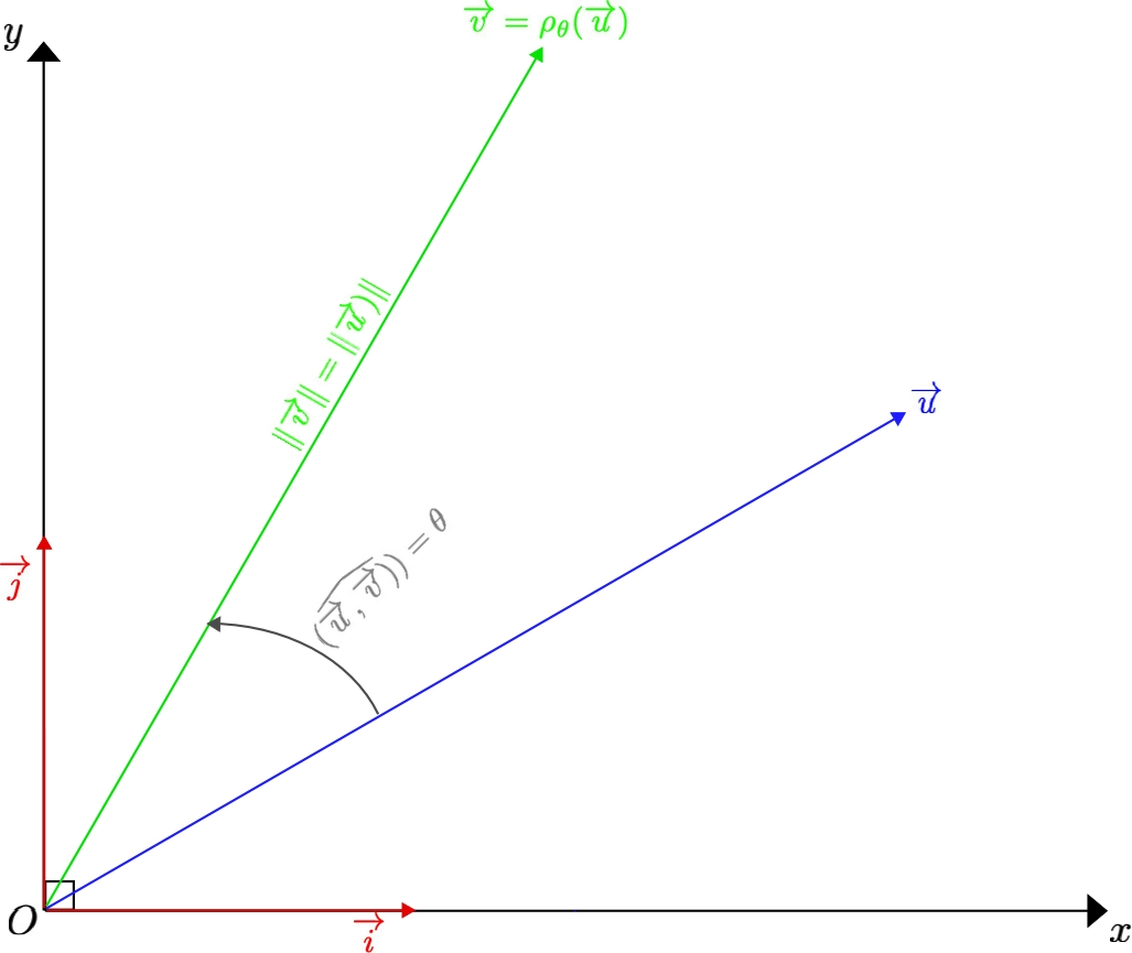
Definition 2
Assume \( \theta\in\mathbb{R}\) is a real number and assume \( \overrightarrow{u}\in\mathbb{P}^*\) is a non-zero vector.
Then the rotated of angle \( \theta\) of the vector \( \overrightarrow{u}\) is the vector \( \overrightarrow{v}\) such as:
\( \left\| \overrightarrow{v} \right\|=\left\| \overrightarrow{u} \right\|\)
\( \widehat{(\overrightarrow{u},\overrightarrow{v})}=\theta\)
Definition 3
Assume \( \theta\in\mathbb{R}\) is a real number.
Then the rotation of angle \( \theta\) is the map \( \rho_{\theta}\) from the euclidean plane \( \mathbb{P}\) to itself, defined as follows:
\( \rho_{\theta}(\overrightarrow{0})=\overrightarrow{0}\) ,
and for any non zero vector \( \overrightarrow{u}\in\mathbb{P}^*\) , \( \rho_{\theta}(\overrightarrow{u})\) is the rotated of angle \( \theta\) of the vector \( \overrightarrow{u}\) .
Theorem 3
The following properties of the rotations hold:
The rotation \( \rho_{0}\) is the identity mapping.
The rotation \( \rho_{pi}\) transforms a vector in its opposite.
For any \( \theta\in\mathbb{R}\) , the application \( \rho_{\theta}\) is one-to-one and its inverse is \( \rho_{\theta}^{-1}=\rho_{(-\theta)}\) .
Proof
Assume \( (\overrightarrow{u},\overrightarrow{v})\in(\mathbb{P}^*)^{2}\) is a non-zero vector.
\( \rho_{0}(\overrightarrow{0})=\overrightarrow{0}\) and, as \( (\widehat{\overrightarrow{u},\overrightarrow{u}})=0\) , \( \rho_{0}(\overrightarrow{u})=\overrightarrow{u}\) .
\( \rho_{\pi}(\overrightarrow{0})=\overrightarrow{0}=-\overrightarrow{0}\) and, as \( (\widehat{\overrightarrow{u},-\overrightarrow{u}})=\pi\) , \( \rho_{\pi}(\overrightarrow{u})=-\overrightarrow{u}\) .
\( \rho_{\theta}(\overrightarrow{0})=\overrightarrow{0}\) and \( \rho_{-\theta}(\overrightarrow{0})=\overrightarrow{0}\) .
Moreover, as \( (\widehat{\overrightarrow{v},\overrightarrow{u}})=-\widehat{(\overrightarrow{u},\overrightarrow{v}})\) , if \( \rho_{\theta}(\overrightarrow{u})=\overrightarrow{v}\) , then \( \rho_{-\theta}(\overrightarrow{v})=\overrightarrow{u}\) .
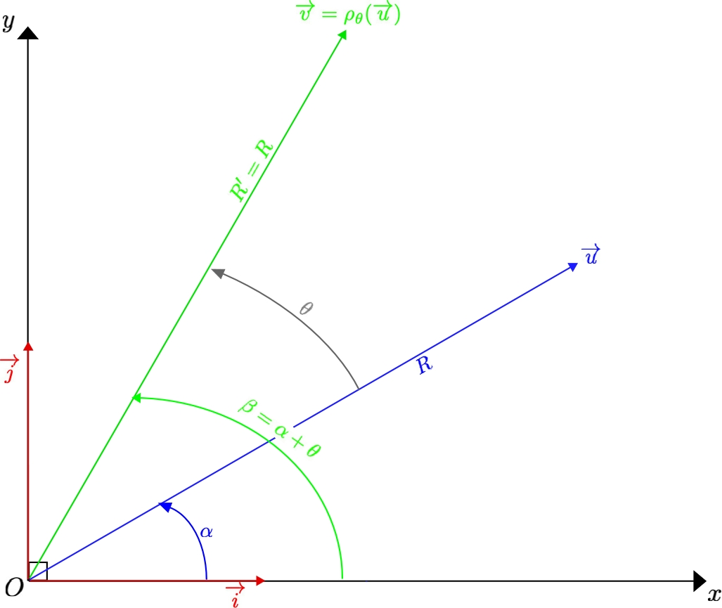
Theorem 4
Assume \( \overrightarrow{u}\in\mathbb{P}^*\) is a non-zero vector with polar coordinates \( (R,\alpha)\) .
Assume \( \overrightarrow{v}\in\mathbb{P}^*\) is a non-zero vector with polar coordinates \( (R',\beta)\) .
Assume \( \overrightarrow{v}=\rho_{\theta}(\overrightarrow{u})\) .
Then the following assertions hold:
\( R'=R\) ,
and \( \beta=\alpha+\theta\) modulo \( 2\pi\) .
Proof
Assume \( \overrightarrow{u}\in\mathbb{P}^*\) is a non-zero vector with polar coordinates \( (R,\alpha)\) .
Assume \( \overrightarrow{v}\in\mathbb{P}^*\) is a non-zero vector with polar coordinates \( (R',\beta)\) .
Assume \( \overrightarrow{v}=\rho_{\theta}(\overrightarrow{u})\) .
Then, as \( \left\| \overrightarrow{v} \right\|=\left\| \overrightarrow{u} \right\|\) , \( R'=R\) .
Moreover, as \( \alpha=\widehat{(\overrightarrow{i},\overrightarrow{u})}\) , \( \beta=\widehat{(\overrightarrow{i},\overrightarrow{v})}\) and \( \theta=\widehat{(\overrightarrow{u},\overrightarrow{v})}\) , then \( \beta=\alpha+\theta modulo \( 2\pi\) \) .
Definition 4
The composed map \( f\circ g\) of two maps \( f\) and \( g\) from \( \mathbb{P}\) to \( \mathbb{P}\) is the map in that, to any vector \( \overrightarrow{u}\in\mathbb{P}\) assigns the vector \( (f\circ g)(\overrightarrow{u})=f(g(\overrightarrow{u}))\) .
Theorem 5
Assume \( (\theta,\mu)\in\mathbb{R}^2\) are real numbers.
Consider the rotation \( \rho_{\theta}\) of angle \( \theta\) and the rotation \( \rho_{\mu}\) of angle \( \mu\) .
Then \( \rho_{\mu}\circ\rho_{\theta}=\rho_{(\theta+\mu)}\) .
Corollary 1
The set of the rotations in \( \mathbb{P}\) with the composition of maps is a commutative group.
Proof (of the theorem 5)
Assume \( (\theta,\mu,R,\alpha)\in\mathbb{R}^4\) are real numbers, and assume \( \overrightarrow{u}\in\mathbb{P}^*\) is a non-zero vector with polar coordinates \( (R,\alpha)\) .
Then the following assertions hold:
The non-zero vector \( \overrightarrow{v}=\rho_{\mu}(\overrightarrow{u})\) has the polar coordinates \( (R,\alpha+\theta)\) .
The non-zero vector \( \overrightarrow{w}=\rho_{\mu}(\overrightarrow{v})\) has the polar coordinates \( (R,\alpha+\theta+\mu)\) .
Consequently, \( \overrightarrow{w}=\rho_{(\theta+\mu)}(\overrightarrow{u})\) .
But \( \overrightarrow{w}=(\rho_{\mu}\circ\rho_{\theta})(\overrightarrow{u})\) .
Consequently, \( (\rho_{\mu}\circ\rho_{\theta})(\overrightarrow{u})=\rho_{(\theta+\mu)}(\overrightarrow{u})\) , and this is true for any non-zero vector \( \overrightarrow{u}\in\mathbb{P}^*\) .
Moreover, \( (\rho_{\mu}\circ\rho_{\theta})(\overrightarrow{0})=\rho_{\mu}(\overrightarrow{0})=\overrightarrow{0}\) and \( \rho_{(\theta+\mu)}(\overrightarrow{0})=\overrightarrow{0}\) as well.
Consequently, \( \rho_{\mu}\circ\rho_{\theta}=\rho_{(\theta+\mu)}\) .
Proof (of the corollary 1)
Assume \( (\theta,\mu,\lambda)\in\mathbb{R}^3\) are real numbers.
Then the following properties may be proved.
Commutativity of \( \circ\) : Because of the commutativity of the addition in \( \mathbb{R}\) :
\( \rho_{\mu}\circ\rho_{\theta}=\rho_{(\theta+\mu)}=\rho_{\mu+\theta}=\rho_{\theta}\circ\rho_{\mu}\)
Associativity of \( \circ\) : Because of the associativity of the addition in \( \mathbb{R}\) :
\( (\rho_{\lambda}\circ\rho_{\mu})\circ\rho_{\theta}=\rho_{(\mu+\lambda)}\circ\rho_{\theta} =\rho_{\theta+(\mu+\lambda)}=\rho_{(\theta+\mu)+\lambda} =\rho_{\lambda}\circ\rho_{\theta+\mu}=\rho_{\lambda}\circ(\rho_{\mu}\circ\rho_{\theta})\)
Neutral element \( \rho_{0}=\text{Id}_{\mathbb{P}}\) for \( \circ\) :
Because \( 0\) is neutral for the addition in \( \mathbb{R}\) : \( \text{Id}_{\mathbb{P}}\circ\rho_{\theta}=\rho_{0}\circ\rho_{\theta}=\rho_{\theta+0}=\rho_{\theta}\)
The inverse of \( \rho_{\theta}\) for \( \circ\) is \( \rho_{\theta}^{-1}=\rho_{(-\theta)}\) :
Because \( -\theta\) is the opposite (additive inverse) of \( \theta\) in \( \mathbb{R}\) : \( \rho_{\theta}^{-1}\circ\rho_{\theta}=\rho_{-\theta}\circ\rho_{\theta}=\rho_{\theta+(-\theta)} =\rho_{0}=\text{Id}_{\mathbb{P}}\)
Consequently, the set of the rotations in \( \mathbb{P}\) with the composition of maps is a commutative group.
You discovered in that note the power of the polar coordinates of non-zero vectors in the euclidean plane \( \mathbb{P}\) to manipulate angles of vectors and to define and manipulate the rotations in \( \mathbb{P}\) .
And now, you are ready for another poweful application of the polar coordinates: the definition and multiplication of the complex numbers in their set \( \mathbb{C}\) .